Field Experiments II
POLSCI 4SS3
Winter 2024
Last time
We learned about implementing field experients
Lots of details!
Sometimes cannot randomly assign
(stepped-wedge design)Today: Thinking about how to do better
Why do better?
Conducting research is expensive
Field experiments are very expensive
Even if you had the resources, we have a mandate to do better
Research ethics
Belmont report: Benefits should outweigh costs
: Researchers have duties beyond getting review board approval
At a minimum, participating in a study takes time
Mandate: Find the most efficient, ethical study before collecting data
Sometimes that means doing more with a smaller sample
Improving Precision
Two ways to improve precision
\[ SE(\widehat{ATE}) =\\ \sqrt{\frac{\text{Var}(Y_i(0)) + \text{Var}(Y_i(1)) + 2\text{Cov}(Y_i(0), Y_i(1))}{N-1}} \]
Two ways to improve precision
\[ SE(\widehat{ATE}) =\\ \sqrt{\frac{\text{Var}(Y_i(0)) + \text{Var}(Y_i(1)) + 2\text{Cov}(Y_i(0), Y_i(1))}{\color{#ac1455}{N-1}}} \]
- Increase sample size Make denominator larger
Two ways to improve precision
\[ SE(\widehat{ATE}) =\\ \sqrt{\frac{\color{#ac1455} {\text{Var}(Y_i(0)) + \text{Var}(Y_i(1)) + 2\text{Cov}(Y_i(0), Y_i(1))}}{N-1}} \]
- Alternative research design Make numerator smaller
Pre-post design
. . .
Outcomes are measured at least twice
Once before treatment, once after treatment
. . .
| Condition | \(t=1\) | Treatment | \(t=2\) |
|---|---|---|---|
| \(Z_i=1\) | \(Y_{i, t=1}\) | X | \(Y_{i, t=2}(1)\) |
| \(Z_i=0\) | \(Y_{i, t=1}\) | \(Y_{i, t=2}(0)\) |
AKA repeated measures design
How does this work?
. . .
- Standard ATE estimator:
\[ E[Y_i(1) | Z_i = 1] - E[Y_i(0) | Z_i = 0] \]
. . .
- Pre-post ATE estimator:
\[ E[(Y_{i,t=2}(1) - Y_{i,t=1}) | Z_i = 1] - E[(Y_{i,t=2}(0) - Y_{i,t=1}) | Z_i = 0] \]
How does this work?
- Standard ATE estimator:
\[ E[Y_i(1) | Z_i = 1] - E[Y_i(0) | Z_i = 0] \]
- Pre-post ATE estimator:
\[ E[(Y_{i,t=2}(1) \color{#ac1455} {- Y_{i,t=1}}) | Z_i = 1] - E[(Y_{i,t=2}(0) \color{#ac1455} {- Y_{i,t=1}}) | Z_i = 0] \]
. . .
- We improve precision by subtracting the variation in the outcome that is unrelated to the treatment
Reasons to use pre-post design
- To increase precision in ATE estimates
. . .
- Most useful when pre-treatment outcomes correlate highly with post-treatment outcomes
. . .
- Problematic when:
. . .
- Pre-treatment outcomes correlate with potential outcomes
- Measuring pre-treatment outcomes leads to attrition
Block randomization
Change how randomization happens
Group units in blocks or strata
Estimate average treatment effect within each
Aggregate with a weighted average
How does it work?
. . .
- Within-block ATE estimator:
\[ \widehat{ATE}_b = E[Y_{ib}(1) | Z_{ib} = 1] - E[Y_{ib}(0) | Z_{ib} = 0] \]
How does it work?
- Within-block ATE estimator:
\[ \widehat{ATE}_\color{#ac1455}b = E[Y_{i\color{#ac1455}b}(1) | Z_{i\color{#ac1455}b} = 1] - E[Y_{i\color{#ac1455}b}(0) | Z_{i\color{#ac1455}b} = 0] \]
. . .
- Overall ATE estimator:
\[ \widehat{ATE}_{\text{Block}} = \sum_{b=1}^B \frac{n_b}{N} \widehat{ATE}_b \]
Illustration
| ID | Block | \(Y_i(0)\) | \(Y_i(1)\) |
|---|---|---|---|
| 1 | 1 | 1 | 4 |
| 2 | 1 | 2 | 5 |
| 3 | 1 | 1 | 4 |
| 4 | 1 | 2 | 5 |
| 5 | 2 | 3 | 8 |
| 6 | 2 | 4 | 9 |
| 7 | 2 | 3 | 8 |
| 8 | 2 | 4 | 9 |
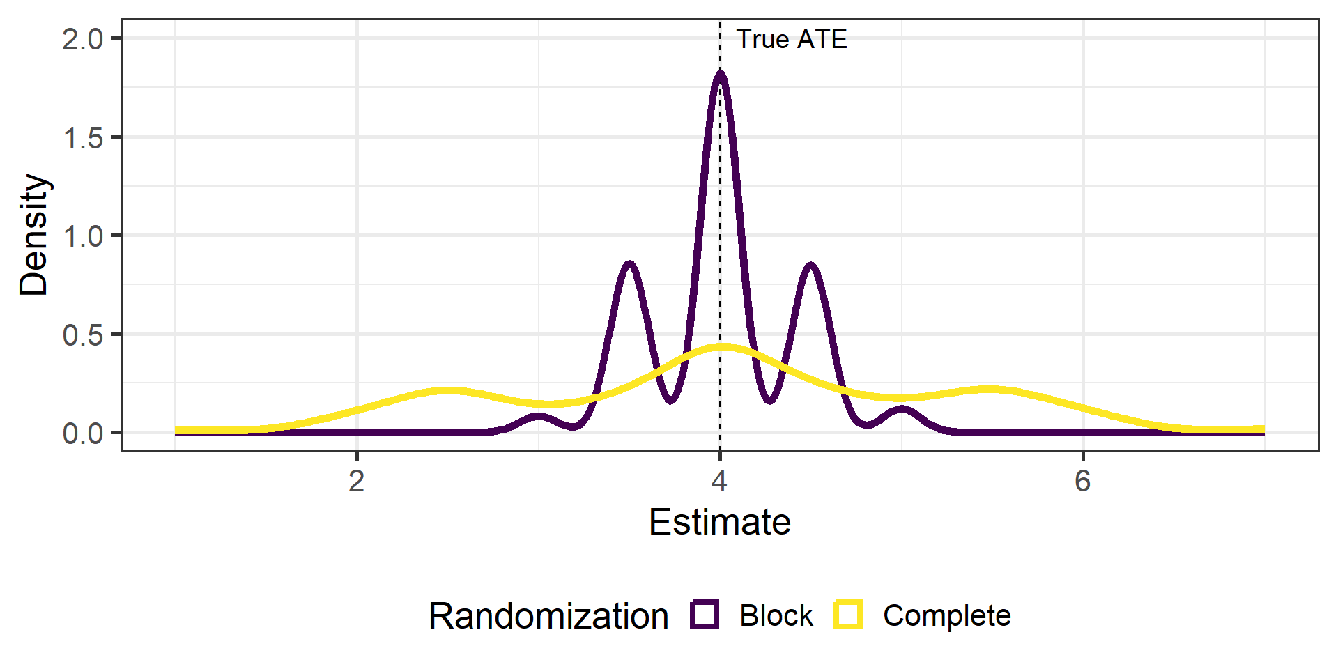
Potential outcomes correlate with blocks
True \(ATE = 4\)
Do 500 experiments
Compare complete and block-randomized experiment
Simulation

Block randomization yields a narrower distribution of estimates
Reasons to block randomize
To increase precision in ATE estimates
To account for possible heterogeneous treatment effects
. . .
Most useful when blocking variables correlate with potential outcomes
And it rarely hurts when they do not correlate!
(more in the lab!)
Example
Kalla et al (2018): Are You My Mentor?
Correspondence experiment with \(N = 8189\) legislators in the US
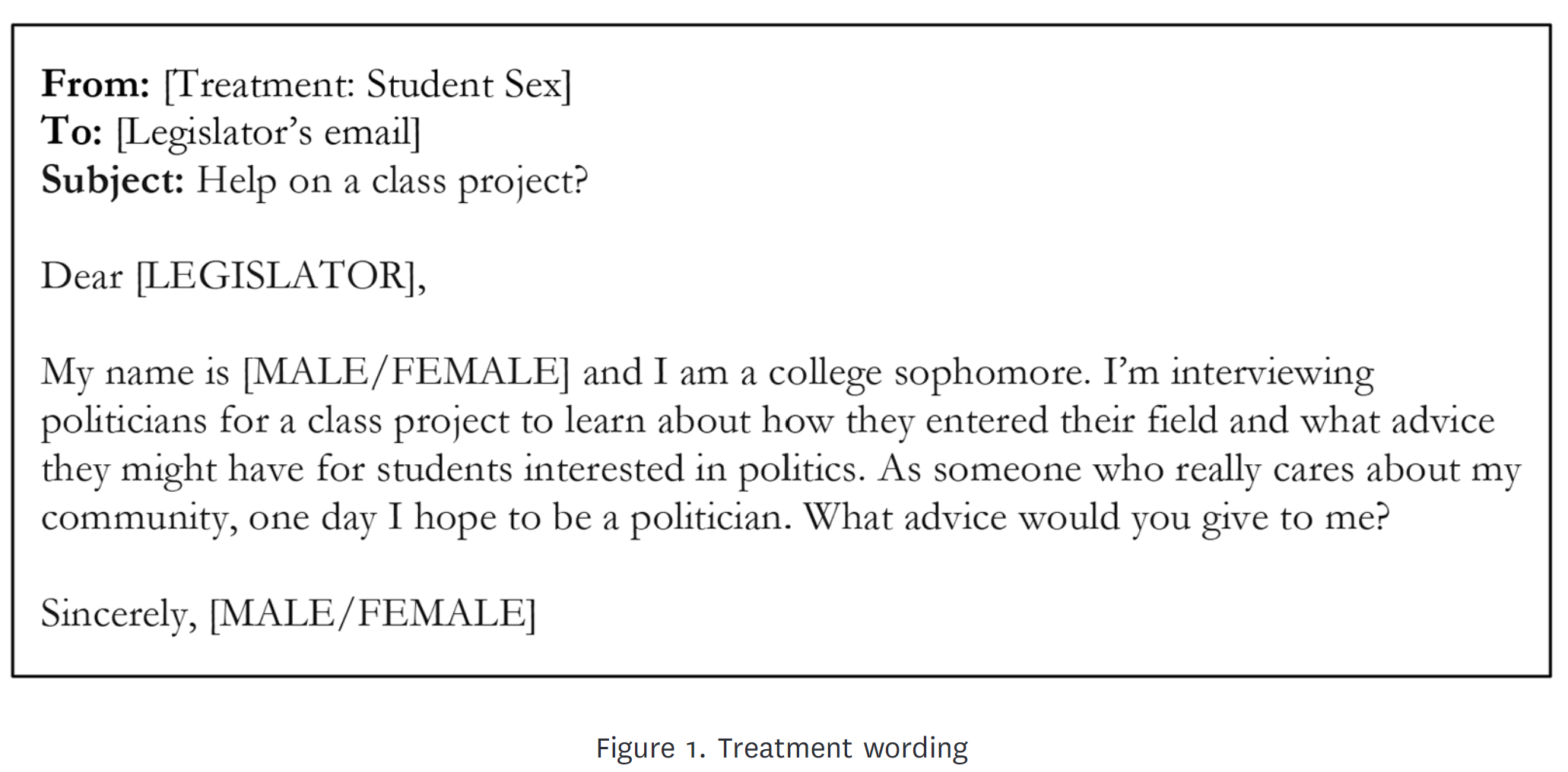
Send email about fake student seeking advice to become politician
Cue gender with student’s name
Also called audit experiments since they were originally designed to audit how responsive elected officials are
Sample email

Data strategy
Block-randomize by legislator’s gender
(why?)Outcomes: Reply content and length
Findings
| Outcome | Male Sender | Female Sender | p-value |
|---|---|---|---|
| Received reply | 0.25 | 0.27 | 0.15 |
| Meaningful response | 0.11 | 0.13 | 0.47 |
| Praised | 0.05 | 0.06 | 0.17 |
| Offer to help | 0.03 | 0.05 | 0.09 |
| Warned against running | 0.01 | 0.02 | 0.14 |
| Substantive advice | 0.07 | 0.08 | 0.33 |
| Word count (logged) | 1.00 | 1.10 | 0.06 |
| Character count | 145.00 | 170.00 | 0.04 |
. . .
- Why not much difference by gender?
Adapted from Table 1
Break time!
