Survey Experiments
POLSCI 4SS3
Winter 2024
Last week
. . .
We discussed and explored techniques to reduce sensitivity bias
Some techniques are observational
(e.g. randomized response)Some techniques are experimental
(e.g. list experiment)Today: Discuss surveys using experiments more generally
Survey experiments
Return to parallels
| Theory | Empirics |
|---|---|
| Model | Data strategy |
| Inquiry | Answer strategy |
Return to parallels
| Theory | Empirics |
|---|---|
| Model | Data strategy |
| Inquiry | Answer strategy |
Types of survey research design
| Inquiry | Observational | Experimental |
|---|---|---|
| Descriptive | Sample survey | List experiment |
| Causal | Panel survey | Survey experiment |
Types of survey research design
| Inquiry | Observational | Experimental |
|---|---|---|
| Descriptive | Sample survey | List experiment |
| Causal | Panel survey | Survey experiment |
Types of survey research design
| Inquiry | Observational | Experimental |
|---|---|---|
| Descriptive | Sample survey | List experiment |
| Causal | Panel survey | Survey experiment |
Types of survey research design
| Inquiry | Observational | Experimental |
|---|---|---|
| Descriptive | Sample survey | List experiment |
| Causal | Panel survey | Survey experiment |
Types of survey research design
| Inquiry | Observational | Experimental |
|---|---|---|
| Descriptive | Sample survey | List experiment |
| Causal | Panel survey | Survey experiment |
. . .
Survey experiments are experimental data strategies that answer a causal inquiry
Technically, list experiments are survey experiments too.
Survey experiments
Assign respondents to conditions or treatments
Usually by random assignment
Each condition is a different version of a question or vignette
Goal: Understand the effect of different conditions on the outcome question if interest
How does this work?
Taking a step back
- Two ways to express functional relations in a model
. . .
Structural causal models
Potential outcomes framework
Taking a step back
- Two ways to express functional relations in a model
Structural causal models
Potential outcomes framework
Potential outcomes framework
Notation
\(i\): unit of analysis
(e.g. individuals, schools, countries)\(Z_i = \{0,1\}\) indicates a condition
(1: Treatment, 0: Control)\(Y_i(Z_i)\) is the individual potential outcome
\(Y_i(0)\): Potential outcome under control
\(Y_i(1)\): Potential outcome under treatment
Toy example
| ID | Female | \(Y_i(1)\) | \(Y_i(0)\) |
|---|---|---|---|
| 1 | 0 | 0 | 0 |
| 2 | 0 | 1 | 0 |
| 3 | 1 | 1 | 0 |
| 4 | 1 | 1 | 1 |
. . .
- \(\tau_i = Y_i(1) - Y_i(0)\) is the individual causal effect
Toy example
| ID | Female | \(Y_i(1)\) | \(Y_i(0)\) | \(\tau_i\) |
|---|---|---|---|---|
| 1 | 0 | 0 | 0 | 0 |
| 2 | 0 | 1 | 0 | 1 |
| 3 | 1 | 1 | 0 | 1 |
| 4 | 1 | 1 | 1 | 0 |
- \(\tau_i = Y_i(1) - Y_i(0)\) is the individual causal effect
. . .
- \(\tau = (1/n) \sum_{i=1}^n \tau_i = E[\tau_i]\) is the inquiry or estimand
. . .
- We call \(\tau\) the Average Treatment Effect (ATE)
Notation chart
Greek
Letters like \(\mu\) denote estimands
A hat \(\hat{\mu}\) denotes estimators
Latin
Letters like \(X\) denote actual variables in our data
A bar \(\bar{X}\) denotes an estimate calculated from our data
\(X \rightarrow \bar{X} \rightarrow \hat{\mu} \xrightarrow{\text{hopefully!}} \mu\)
\(\text{Data} \rightarrow \text{Estimate} \rightarrow \text{Estimator} \xrightarrow{\text{hopefully!}} \text{Estimand}\)
Challenge
We want to know the ATE \(\tau\)
This requires us to know \(\tau_i = Y_i(1) - Y_i(0)\)
But when we assign treatment conditions we only observe one of the potential outcomes \(Y_i(1)\) or \(Y_i(0)\)
Meaning that \(\tau_i\) is impossible to calculate!
This is the fundamental problem of causal inference
Continuing the example
| ID | Female | \(Y_i(1)\) | \(Y_i(0)\) | \(\tau_i\) |
|---|---|---|---|---|
| 1 | 0 | 0 | 0 | 0 |
| 2 | 0 | 1 | 0 | 1 |
| 3 | 1 | 1 | 0 | 1 |
| 4 | 1 | 1 | 1 | 0 |
. . .
- We can randomly assign conditions \(Z_i\)
Continuing the example
| ID | Female | \(Y_i(1)\) | \(Y_i(0)\) | \(\tau_i\) | \(Z_i\) | \(Y_i\) |
|---|---|---|---|---|---|---|
| 1 | 0 | 0 | 0 | 0 | 1 | 0 |
| 2 | 0 | 1 | 0 | 1 | 0 | 0 |
| 3 | 1 | 1 | 0 | 1 | 1 | 1 |
| 4 | 1 | 1 | 1 | 0 | 0 | 1 |
. . .
We observe outcome \(Y_i\) depending on assigned condition \(Z_i\)
We can use this to approximate the ATE with an estimator
Estimator for the ATE
- Additive property of expectations:
\[ \tau = E[\tau_i] = E[Y_i(1) - Y_i(0)] \\ = \underbrace{E[Y_i(1)] - E[Y_i(0)]}_{\text{Difference in means between potential outcomes}} \]
. . .
- We cannot calculate this, but we can calculate
\[ \hat{\tau} = \underbrace{E[Y_i(1) | Z_i = 1] - E[Y_i(0) | Z_i = 0]}_{\text{Difference in means between conditions}} \]
Randomization
If we can claim that units are selected into conditions \(Z_i\) independently from potential outcomes
Then we can claim that \(\hat{\tau}\) is a valid approximation of \(\tau\)
In which case we say that \(\hat{\tau}\) is an unbiased estimator of the ATE
Random assignment of units into conditions guarantees this in expectation
Discussion
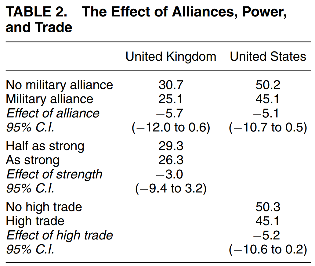
Tomz and Weeks (2013): “Public Opinion and the Democratic Peace”
Surveys in the UK (\(n = 762\)) and US (\(n = 1273\))
April-May 2010
Outcome: Support for military strike
2x2x2 survey experiment
Vignette design
. . .
UK
Political regime: Democracy/not a democracy
Military alliances: Ally/not an ally
Military power: As strong/half as strong
US
Political regime: Democracy/not a democracy
Military alliances: Ally/not an ally
Trade: High level/not high level
Results for democracy

Results for other factors

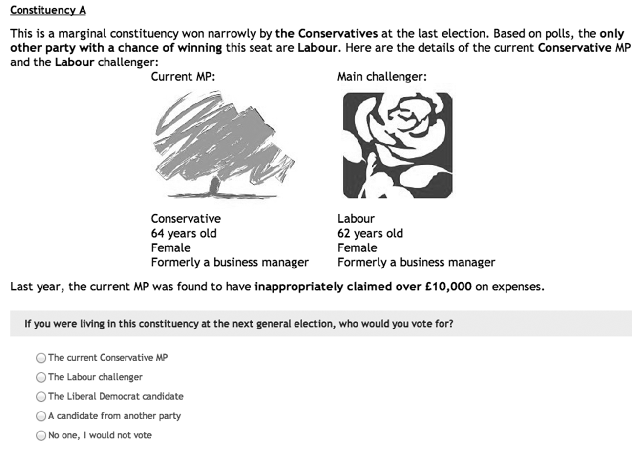
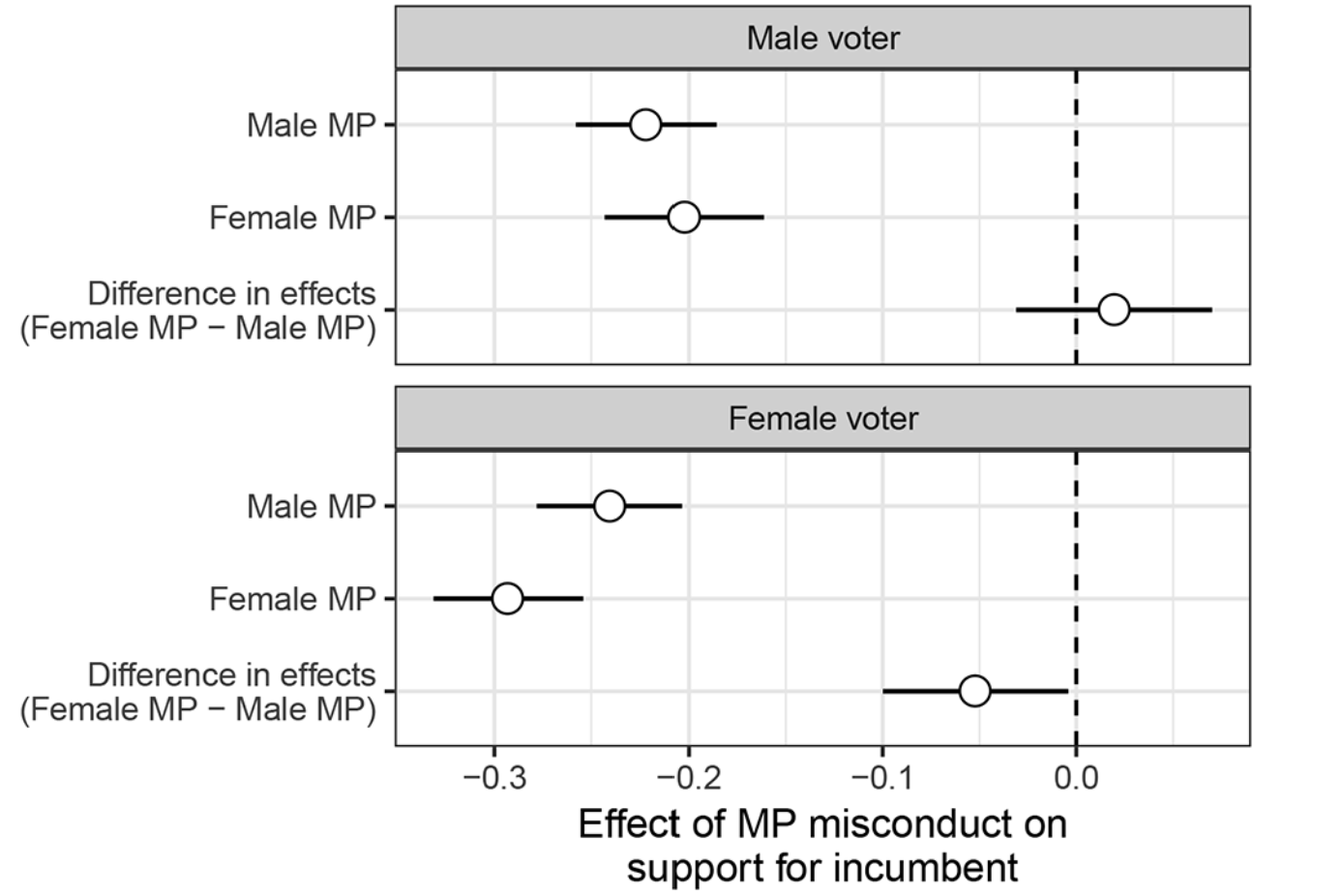
Eggers et al (2017): “Corruption, Accountability, and Gender”
. . .

Profile variants
| Factor | MP | Challenger |
|---|---|---|
| Party | Labour, Conservative | Labour, Conservative, Liberal Democrat |
| Age | 45, 52, 64 | 40, 52, 64 |
| Gender | Male, Female | Male, Female |
| Previous job | General practitioner, journalist, political advisor, teacher, business manager | General practitioner, journalist, political advisor, teacher, business manager |
Results

Next Week
Convenience Samples
Focus on: Should findings generalize?
Break time!
